Increase Related Tags using Graph Modeling Algorithms

This article describes our journey to increase the number of Related Tags offered by Empathy.co to customers and shoppers. But, wait, first things first — what are Related Tags? 🤔

Related Tags are tools that help shoppers streamline their search experience, offering additional terms that are relevant to their query, based upon other recent searches on the same website.

In the image above, we can see that for the query shirt, our engine has offered the Related Tags spring, summer, teal, winter, women and yellow. Essentially, this means that other searches containing the same term were conducted and those were some of the words frequently combined with shirt.

Related Tags are simply additional search terms that contain the same base query.

Cool, we’ve got that cleared up. 🙂 So, how do we calculate them?

It all happens within a session journey. Let’s imagine a shopper entering a website and searching for the following:

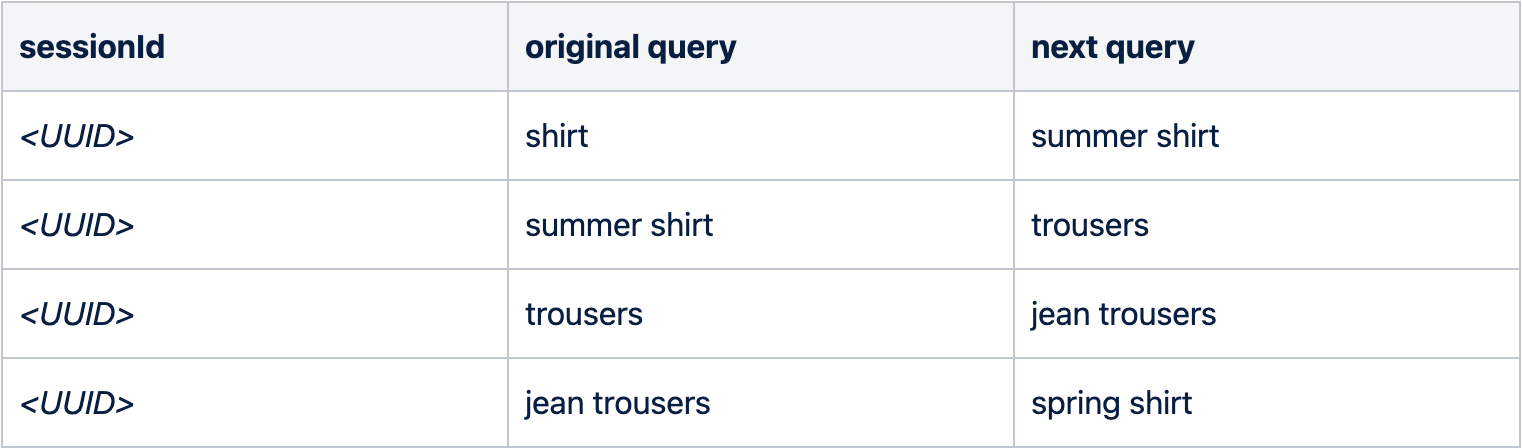
shirt → summer shirt → trousers → jean trousers → spring shirt

That session’s information is then stored in our data lake in the form of direct pairs as original query → next query. It is worth reiterating that Empathy.co is strongly committed to privacy and creates products that are both trustworthy and evoke trust. Therefore, that UUID is nothing but a random identifier that denotes each session uniquely, but it does not contain any personal information.

In this particular example, we would have a file with the following information (along with many other users' sessions):

From those sessions and based on the aforementioned explanation, we are able to calculate the following Related Tags (note that the original query is contained in the next query):

shirt → summer shirt
trousers → jean trousers

However, if we look at the entire session above, we realize there is another Related Tag we would have liked to calculate: shirt → spring shirt

Hold on…why didn’t we calculate it if both of those terms were in the session? Well, the reason is that we are only looking at direct pairs; and because spring shirt was preceded by jean trousers, no direct connection between shirt and spring shirt exists.

Going Beyond Direct Pairs

Once we know what Related Tags are and how they are calculated here at Empathy.co, we want to eliminate the limitation of using only direct pairs. By looking several queries ahead, we are able to increase the step sizes within the session. Our current algorithm to calculate Related Tags is based on Apache Spark batches that run on Kubernetes, using a Spark operator that allows us to decide which cloud provider to use. At the moment, they are running on AWS.

Let’s see how we can overcome that limitation. 😉

Attempt I: Same Approach Using the Entire Session

Rather than fully modifying the algorithm right away, we decided to try a more simple approach: increase the number of steps that are taken into account for the calculation. Therefore, using the initial session we described as an example, the pairs could be adapted to a bigger step size:

shirt → summer shirt (direct pair)
shirt → summer shirt → trousers (step size = 2)
shirt → summer shirt → trousers → jean trousers (step size = 3)
shirt → summer shirt → trousers → jean trousers → spring shirt (step size = 4)

Great! By doing that, we have managed to increase the number of Related Tags simply by multiplying the possibilities that a sequence of next queries will contain the original query. The issue is that when calculating all combinations of all sessions, which is much more expensive, the average increment was not as relevant as initially expected. We had to come up with another option and one of our colleagues had an interesting suggestion: how about storing all these sessions in a graph, in order to benefit from the relationships between terms?

Attempt II: Using a Graph Algorithm

Graph algorithms are often used to solve many distinct problems where data can be presented as nodes that can be linked or connected in the form of relationships. In our domain, queries are represented as nodes and a relationship between one node and another means that a shopper went from original query → next query in a single session. The following image illustrates two sessions from different users, where both queried q1, q2, q3, and q5.

Therefore, if we were to represent this as a graph, the equivalent would be something along these lines:

We can see how nodes q2 - q3 are weighted higher than the rest of the nodes - simply because there were two distinct sessions in which these queries were performed one after the other. From now we can assume there is no distinction between q2 → q3 and q3 → q2.

Data Preparation

Before actually starting with the code, we need to prepare the data. As we mentioned previously, we are going to use sessions from the wisdom of the crowd. To facilitate the bulk insert, instead of having the full session, we have collected all direct pairs and the corresponding count, which is simply how many times a customer went from original query → next query.

To do so, we use a simple JSON model:

[
  {"from": "shirt", "to": "summer shirt", "count": 146},
  {"from": "trousers", "to": "jean trousers", "count": 140},
  {"from": "jean trousers", "to": "spring shirt", "count": 131},
  {...}
]

Easy! All these direct pairs will now be imported into the graph, where from and to will be represented as nodes and the count will represent the weight of that relationship.

In order to facilitate this, we store all the from, to, and count information in a simple data frame that will be used later on in both the Neo4j and Spark GraphX sections.

val defaultInputSchema: StructType = new StructType()
  .add(FROM_COL, StringType)
  .add(TO_COL, StringType)
  .add(COUNT_COL, LongType)

def readEdgeData(sparkSession: SparkSession, schema: StructType, file: String): DataFrame = {
  sparkSession.read.schema(schema).json(file).toDF()
}

Using a Neo4j Database

Now that we’ve decided to explore nodes and relationships using a graph database to represent queries and sessions, it is time to compile the requirements to be satisfied.

Query Capabilities: Although this sounds sort of obvious, we can use any query language (not necessarily SQL-like querying) so that we can extract the Related Tags from the nodes and relationships.
Ability to Set Attributes: As described in the previous section, we are using weights (counts) to sort pairs based on the number of occurrences. Therefore, this is essential to be able to set it at the relationship (edge) level.
Scalability/Performance: Our RT calculation is done via Spark batches, thus, we need a way to scale horizontally if the amount of data increases. This is a limitation in the community edition we are going to use for this POC. We would need to provision the enterprise edition if we decide to go with this solution.

That being said, our choice is to use Neo4j since it satisfies all the requirements listed above. Also, since we are using Apache Spark in Scala, we can benefit from the Neo4j Spark connector as described in the Neo4j Spark documentation.

Data Extraction & Load

Code time! Assuming our edge data is already set up as a data frame, it just needs to be passed over to the Neo4j connector to load the data frame into the database. The code is quite straightforward: the source and target nodes have to be specified, as do the properties. Note that, for the sake of simplicity, we have removed some of the configurations (authentication, database URL, etc). Remember to reference the official Neo4j documentation for more detailed information about all the options.

def loadDataIntoNeo4j(df: DataFrame): Unit = {
  df.write.format("org.neo4j.spark.DataSource")
    // set the relationships between queries
    .option("relationship", "CONNECTS_TO")
    .option("relationship.save.strategy", "keys")
    .option("relationship.source.labels", ":Query")
    .option("relationship.source.node.keys", "from:query")
    .option("relationship.target.labels", ":Query")
    .option("relationship.target.node.keys", "to:query")
    // set the edge weights of the relationship
    .option("relationship.properties", "count:weight")
    // avoid multiple nodes reflecting same query
    .option("schema.optimization.type", "NODE_CONSTRAINTS")
    .save()
}

Ta-dah! 🎉 Now our data has been saved and we can start querying for relationships. The following image shows a representation of the graph for the query top. This is indeed an extremely useful explainability tool and allows us infer information about why a Related Tag was offered based on the data.

Running the Algorithm

All right, the data is ready. In this case, we are going to use Cypher Query Language to run the queries on top of Neo4j. Just like before, we are going to use Spark to issue the query that will calculate the Related Tags. Again, by setting authentication parameters and telling the connector to use the query option we can send any type of query based on CQL.

def executeQuery(sparkSession: SparkSession, query: String): DataFrame = {
  sparkSession.read.format("org.neo4j.spark.DataSource")
    .option("url", Config.appConfig.neo4JUrl)
    .option("query", query)
    .load()
}

Using the following query to calculate the related tags:

val MATCH_RELATED_TAGS_GROUP_BY_STEP_SIZE: String =
  """
    |MATCH p = (from:Query) -[*1..5]-> (to:Query)
    |WITH nodes(p) AS ns, relationships(p) AS rels
    |UNWIND size(rels) AS step_size
    |UNWIND ns[0].query AS from_query
    |UNWIND ns[step_size].query AS to_query
    |WITH ns, rels, from_query, to_query, step_size
    |WHERE from_query <> to_query
    |    AND NONE (n IN tail(ns) WHERE n.query = from_query)
    |    AND ((to_query =~ ('^' + from_query + ' .*$')) OR
    |        (to_query =~ ('^.* ' + from_query + ' .*$')) OR
    |        (to_query =~ ('^.* ' + from_query + '$'))
    |    )
    |WITH DISTINCT from_query AS from, to_query AS to, min(step_size) AS step_size
    |RETURN from, to, step_size
    |ORDER BY step_size
    |""".stripMargin

In a nutshell, this query is evaluating every node that is connected from step sizes 1-5 (relationships in the graph), where the source node is the original query, and the target node is the next query that contains the related tag. Note that we are limiting the algorithm to five relationships to avoid an endless query. 🥳

Conclusion

After running the algorithm in the Neo4j database, we are able to see a considerable increment in the number of Related Tags overall, and also in-depth (not only how many Related Tags we have now vs. the previous algorithm, but how many new Related Tags we have now for the queries that didn't have any in the previous version). The numbers are promising, yet there are some drawbacks when using Neo4j as part of our batch executions.

Need for provisioning and maintaining the database in the cloud.
Idle time. Because our Related Tags calculation is a batch project that runs nightly, there is no real need to have it running 24/7. That means the database may be idle most of the time.
Potential performance bottleneck. Even considering the enterprise version of Neo4j, we cannot really benefit from the Spark parallelization of work if our main algorithm runs in a non-distributed database.
Enterprise pricing 💸

With all those concerns taken into account, our last and final attempt (for now, anyway) was to use Spark Graph utilities to circumvent the aforementioned points.

Using Built-in Spark GraphFrame & Graphx Utilities

Spark GraphX and GraphFrame utilities are almost exactly the same, the only difference being the underlying usage of RDDs and DataFrames, respectively. This makes them quite interesting for our use case, as they give us the same advantages as the database (nodes and relationships, query capabilities, etc). In fact, we don’t need to provision anything new in our cluster nor wonder what performance will be like since we can use the Spark elasticity & parallelization. The other beneficial aspect is that the graph will only be active during the algorithm execution. Therefore, the cost/maintenance of this solution is much more scalable.

Data Extraction & Load

Just as we did in the Neo4j experiment, we need to prepare a from → to → count file with all the candidates that will feed the data frame. The difference, though, is that we are not relying on an intermediate library or connector.

Now, given the pairs data frame, we need to transform it to a GraphX based on Spark RDDs.

def loadDataIntoGraphX(sparkSession: SparkSession, edgeDF: DataFrame): Graph[String, VertexId] = {
  import sparkSession.implicits._
  val distinctFromQueries = edgeDF.select(FROM_COL)
    .distinct()
    .withColumnRenamed(FROM_COL, QUERY_COL)
  val distinctToQueries = edgeDF.select(TO_COL)
    .distinct()
    .withColumnRenamed(TO_COL, QUERY_COL)
  val allDistinctQueries = distinctFromQueries.union(distinctToQueries).distinct()
  
  // add ID
  val windowSpec: WindowSpec = Window.orderBy(QUERY_COL)
  val uniqueQueriesWithID = allDistinctQueries
    .withColumn(ID_COL, row_number.over(windowSpec))

  // transform to map
  val idToQueryMap: Map[Long, String] = uniqueQueriesWithID.select(ID_COL, QUERY_COL).as[(Long, String)].collect().toMap
  val queryToIdMap: Map[String, Long] = uniqueQueriesWithID.select(QUERY_COL, ID_COL).as[(String, Long)].collect().toMap

  // put this into graph structure
  val edgeRDD: Dataset[Edge[Long]] = edgeDF.select(FROM_COL, TO_COL, COUNT_COL).map {
    case Row(fromQuery: String, toQuery: String, weight: Long) => Edge[Long](
      queryToIdMap(fromQuery), queryToIdMap(toQuery), weight)
  }
  // construct the graph
  val graph: Graph[Int, VertexId] = Graph.fromEdges[Int, Long](edgeRDD.rdd, 0)
  
  // mapping the single vertices IDs to their actual queries
  val idToQuery: Long => String = id => idToQueryMap.getOrElse(id, "")
  graph.mapVertices((id, _) => idToQuery(id))
}

Voilà! Our direct pairs collection is now stored as a GraphX RDD in Spark. The idea is to use the data to create two distinct columns, from and to, and then generate the edgeRDD, which creates as many rows as there are pairs in the original file. The final step here is to apply a map function to map each vertex with an identifier.

Sweet! Let’s now calculate the related tags using GraphFrames.

Running the Algorithm

In this case, instead of writing an SQL-like statement, we are benefitting from the Spark functions in order to operate within the data frame (which was first converted to GraphFrame as shown in line 3). The code is quite concise, and the goal is to find all the pairs (no matter the step size) of original query → next query that minimize the number of steps required to find a Related Tag.

def generateCandidates(sparkSession: SparkSession, graph: Graph[String, VertexId]): DataFrame = {
  // convert to GraphFrame (more suitable for queries)
  val graphFrame: GraphFrame = GraphFrame.fromGraphX(graph)
  
  // generate all smaller step sizes, too, apply all the filtering regarding contained loops and the like  
  // then reduce to from, to, and stepSize for RTs, then calculate the unique RTs per stepSize  
  Range(1, Config.appConfig.stepSize, 1).inclusive.foreach(step => {
    val allVerticesQueriesSelectors = Queries.getNodesForNStepQuery(step).map(x => s"$x.attr")
    val dfForStepSize = graphFrame.find(Queries.getNStepQuery(step))
      .withColumn(IS_RT_COLUMN, Queries.isRelatedTagUdf(col(allVerticesQueriesSelectors.head), col(allVerticesQueriesSelectors.last)))
      .filter(col(IS_RT_COLUMN) === true)
      .select(col(allVerticesQueriesSelectors.head).as(FROM_COLUMN), col(allVerticesQueriesSelectors.last).as(TO_COLUMN))
      .withColumn(STEP_SIZE_COLUMN, lit(step.toLong))
      .select(FROM_COLUMN, TO_COLUMN, STEP_SIZE_COLUMN)
    if (Objects.isNull(df)){
      df = dfForStepSize
    }
    else {
      df = df.union(dfForStepSize)
    }
  })
  // now remove duplicates from lower step sizes
  df.groupBy(FROM_COLUMN, TO_COLUMN)
    .agg(min(STEP_SIZE_COLUMN).as(STEP_SIZE_COLUMN))
    .dropDuplicates()
    .orderBy(col(STEP_SIZE_COLUMN).asc)
}

Conclusions

After running the algorithm, we compared all the results with those provided by the Neo4j implementation. Good news! 🎊 The resulting Related Tags are exactly the same and the numbers match. In addition, this solution has some advantages over the database (a few of which have already been mentioned).

No New Provisions: Nope, there’s really no need for anything new. The code can run on either a local machine (without the need to install anything new) or a Spark cluster.
Quick Replacement: This algorithm is able to replace the one currently being used, without any additional consideration. Since both the old and new approaches use Spark, it’s an easy transition.
Performance: Although this solution is not cheap (it’s a lot of computation, indeed), it is able to support larger amounts of data – just add more executors.
Customer Feedback: This goes hand-in-hand with the previous point: if we’re able to evolve the algorithm quickly, then customers will be able to give us feedback sooner.

After considering all the different factors, we decided to use Spark GraphX & GraphFrame as our new Related Tags algorithm. 🏆

Summary

After exploring both approaches using graph algorithms, we want to share some numbers using data from some of our medium-large customers. The final analysis consists of three different but equally insightful metrics.

Increase in Overall Volume: A gross, overall measurement of how many new Related Tags are being produced. Even though this metric is telling us that we are able to increase the related tags by, in some cases, more than 50%, it is not yet very accurate. It may happen (and it actually already so happens), that the increment occurred on original queries that already had a high number of Related Tags. Say we have original query = shirt with 10 Related Tags using the old algorithm. If, after applying this code, we are able to produce 50 new Tags for the term “shirt”, it is not very valuable since we already had quite a few for that term.
Increase in Unique Query Volume: As noted in the previous point, we would really like to know if the algorithm is indeed adding Related Tags to original queries that previously had no tags. In the following picture, we can see that in some cases, up to 47% of queries now have Related Tags. This is a great increment because shoppers are able to see the difference.

Increase Depth for Low-Count Queries: This analysis drills down even further, in order to understand how well the new algorithm is behaving. There are many queries in which the number of Related Tags is very limited (1, 2, or 3). In this case, we are measuring what the increment is, on average, to those queries under the desired number of Tags (we consider 5 to be a reasonably good number). As an example, for Customer 1, there were 150 queries that only had one Related Tag each. After applying the graph algorithm, those queries have an average of 3.59 (+2.59) Tags. If we focus on the 57 queries that had two Related Tags per query, the algorithm subsequently increased the average to 4.7 (+2.7) Tags.

Possible Explorations

Our main concern when deciding whether to opt for the Neo4j implementation or the Spark GraphX was, as previously explained, the architectural requirements (database provisioning/maintenance), quick algorithm replacement, and performance.

However, there are many other aspects worth considering. Using a database will give us some interesting benefits:

Built-in Explainability & Visualization: Neo4j (and other graph-based databases) come with a visualization tool that is ideal for our customers, as it aids in understanding why some related tags are generated, but not others, as well as evaluating the performance of single queries, and much more.
Query Clustering: Queries (nodes) are connected in the form of relationships (edges), which are translated into many small clusters for each original query. This allows additional information to be inferred about how original queries are related.
Attributes Manipulation: Interacting with the attributes within the graph to boost or bury certain queries, affect the weight of a particular relationship, has and allow it to be manipulated.

There are many possibilities to explore, out there.

Hope you’ve found this interesting and helpful! Stay tuned for more articles! 📝

Going Beyond Direct Pairs

Attempt I: Same Approach Using the Entire Session

Attempt II: Using a Graph Algorithm

Data Preparation

Using a Neo4j Database

Data Extraction & Load

Running the Algorithm

Conclusion

Using Built-in Spark GraphFrame & Graphx Utilities

Data Extraction & Load

Running the Algorithm

Conclusions

Summary

Possible Explorations

Versions Used